STRUKTUR MODAL SLIDE BRIGHAM DIMODIFIKASI OLEH

Presentasi berjudul: "STRUKTUR MODAL SLIDE BRIGHAM DIMODIFIKASI OLEH"— Transcript presentasi:

1 STRUKTUR MODAL SLIDE BRIGHAM DIMODIFIKASI OLEH
DR. KHAIRA AMALIA F, SE.AK, CA, MBA, MAPPI (CERT)

2 CAPITAL STRUCTURE Bauran hutang dan ekuitas untuk pendanaan perusahaan Bauran debt dan equity (Brigham dan Daves, 2004) Hutang jangka pendek yang bersifat permanen, hutang jangka panjang, dan modal sendiri (preferen dan saham biasa)

3 CAPITAL STRUCTURE VS FINANCIAL STRUCTURE
CS = noncurrent liabilities + preferred equity + common equity FS = Capital Structure + Current liabilities (Keown et al)

4 Hubungan dengan Biaya Modal
Struktur modal mempengaruhi biaya modal (cost of capital) Perhitungan Coc diperlukan untuk: Maksimalisasi Nilai Perusahaan yang memerlukan biaya modal minimum Keputusan Penganggaran Modal (Capital Budgeting)

5 Struktur Modal dan Nilai Perusahaan
Nilai perusahaan bila dijual Nilai dicerminkan harga saham Ada beberapa model

6 Who are Modigliani and Miller (MM)?*
They published theoretical papers that changed the way people thought about financial leverage. They won Nobel prizes in economics because of their work. MM’s papers were published in 1958 and Miller had a separate paper in The papers differed in their assumptions about taxes.

7 What assumptions underlie the MM and Miller models?*
Firms can be grouped into homogeneous classes based on business risk. Investors have identical expectations about firms’ future earnings. There are no transactions costs. (More...)

8 All debt is riskless, and both individuals and corporations can borrow unlimited amounts of money at the risk-free rate. All cash flows are perpetuities. This implies perpetual debt is issued, firms have zero growth, and expected EBIT is constant over time. (More...)

9 Asumsi MM tanpa pajak Tidak ada pajak pribadi maupun pajak perusahaan Resiko bisnis dapat diukur dengan deviasi standar EBIT Seluruh investor memiliki estimasi yang sama tentang EBIT perusahaan di masa yang akan datang

10 Saham dan obligasi diperdagangkan di pasar modal yang sempurna
Hutang perusahaan dan individu tanpa resiko, sehingga suku bunga hutang adalah suku bunga bebas resiko Seluruh aliran kas adalah perpetuitas, dengan kata lain

11 Pertumbuhan perusahaan adalah nol atau EBIT selalu konstan

12 MM’s first paper (1958) assumed zero taxes. Later papers added taxes.
No agency or financial distress costs. These assumptions were necessary for MM to prove their propositions on the basis of investor arbitrage.

13 rsL = rsU + (rsU - rd)(D/S).
MM with Zero Taxes (1958) Nilai perusahaan tidak tergantung pakai hutang or not atau tidak tergantung struktur modal Proposition I: VL = VU. Proposition II: rsL = rsU + (rsU - rd)(D/S).

14 VL = VU = EBIT = EBIT WACC KSU Nilai Perusahaan V = D + S Dalam dunia tanpa pajak WACC = KSU rsL = rsU + (rsU - rd)(D/S).

15 Given the following data, find V, S, rs, and WACC for Firms U and L.
Firms U and L are in same risk class. EBITU,L = $500,000. Firm U has no debt; rsU = 14%. Firm L has $1,000,000 debt at rd = 8%. The basic MM assumptions hold. There are no corporate or personal taxes.

16 1. Find VU and VL. EBIT rsU $500,000 0.14 VU = = = $3,571,429. VL = VU = $3,571,429. Questions: What is the derivation of the VU equation? Are the MM assumptions required?

17 2. Find the market value of Firm L’s debt and equity.
VL = D + S = $3,571,429 $3,571,429 = $1,000,000 + S S = $2,571,429.

18 3. Find rsL. rsL = rsU + (rsU - rd)(D/S) = 14.0% + (14.0% - 8.0%)( ) = 14.0% % = 16.33%. $1,000,000 $2,571,429

19 4. Proposition I implies WACC = rsU.
Verify for L using WACC formula. WACC = wdrd + wcers = (D/V)rd + (S/V)rs = ( )(8.0%) +( )(16.33%) = 2.24% % = 14.00%. Rsu tadi 14.00% juga kan… $1,000,000 $3,571,429 $2,571,429 $3,571,429

20 Graph the MM relationships between capital costs and leverage as measured by D/V.
Without taxes Cost of Capital (%) 26 20 14 8 rs WACC rd Debt/Value Ratio (%)

21 Sjahrial p.130: Pada saat keseimbangan, nilai perush U dan L serta WACC sama. Proses arbitrase terjadi karena jika nilai L tinggi sahamnya akan dijual dan harga saham akan turun. Pembelian saham U akan menyebabkan nilainya naik. So, nilai pasar kedua perusahaan akan sama

22 The more debt the firm adds to its capital structure, the riskier the equity becomes and thus the higher its cost. Although rd remains constant, rs increases with leverage. The increase in rs is exactly sufficient to keep the WACC constant.

23 Graph value versus leverage.
Value of Firm, V (%) 4 3 2 1 VU VL Firm value ($3.6 million) Debt (millions of $) With zero taxes, MM argue that value is unaffected by leverage.

24 Contoh UT Tidak ada pajak D = 0 S = Rp EBIT =

25 Apabila perusahaan tidak berhutang maka biaya modal sendiri KSU = 12% bila berhutang Kd = 8%, dan uang pinjaman digunakan untuk membeli kembali saham, dkl bila hutang bertambah sebesar X maka modal sendiri akan berkurang sebesar X pula sehingga aktiva atau nilai perusahaan konstan

26 Vu = EBIT / Ksu = / 12% = Rp D = Rp S = V-D S = – = maka

27 rsL = rsU + (rsU - rd)(D/S)
= 12% + (12% - 8.0%) x ( / ) = 12% + 4% = 16%. WACC =

28 = 4% + 8%% = 12.00%. Rsu tadi 12.00% juga kan…
WACC = wdrd + wcers = (D/V)rd + (S/V)rs = ( / )(8.0%) +( / )(16%) = 4% + 8%% = 12.00%. Rsu tadi 12.00% juga kan…

29

30 VL = VU + TD. rsL = rsU + (rsU - rd)(1 - T)(D/S).
MM dengan Pajak WACC u > WACC L UT nilai < Find V, S, rs, and WACC for Firms U and L assuming a 40% corporate tax rate. With corporate taxes added, the MM propositions become: Proposition I: VL = VU + TD. Proposition II: rsL = rsU + (rsU - rd)(1 - T)(D/S).

31 Notes About the New Propositions
1. When corporate taxes are added, VL  VU. VL increases as debt is added to the capital structure, and the greater the debt usage, the higher the value of the firm. 2. rsL increases with leverage at a slower rate when corporate taxes are considered.

32 1. Find VU and VL. EBIT(1 - T) rsU $500,000(0.6) 0.14
Note: Represents a 40% decline from the no taxes situation. VL = VU + TD = $2,142, ($1,000,000) = $2,142,857 + $400,000 = $2,542,857.

33 2. Find market value of Firm L’s debt and equity.
VL = D + S = $2,542,857 $2,542,857 = $1,000,000 + S S = $1,542,857.

34 3. Find rsL. rsL = rsU + (rsU - rd)(1 - T)(D/S)
= 14.0% + (14.0% - 8.0%)(0.6)( ) = 14.0% % = 16.33%. $1,000,000 $1,542,857

35 WACCL = (D/V)rd(1 - T) + (S/V)rs = ( )(8.0%)(0.6) +( )(16.33%)
4. Find Firm L’s WACC. WACCL = (D/V)rd(1 - T) + (S/V)rs = ( )(8.0%)(0.6) +( )(16.33%) = 1.89% % = 11.80%. When corporate taxes are considered, the WACC is lower for L than for U. $1,000,000 $2,542,857 $1,542,857 $2,542,857

36 MM relationship between capital costs and leverage when corporate taxes are considered.
Cost of Capital (%) rs 26 20 14 8 WACC rd(1 - T) Debt/Value Ratio (%)

37 MM relationship between value and debt when corporate taxes are considered.
Value of Firm, V (%) 4 3 2 1 VL TD VU Debt (Millions of $) Under MM with corporate taxes, the firm’s value increases continuously as more and more debt is used.

38 Contoh UT 6.11 Ada pajak EBIT = T=40%, D=0 data lain sama Vu = EBIT(1 - T) rsU Vu = (1-40%) / 0.12 Vu = Rp

39 VL = VU + TD = (40% x ) = maka V = S + D = S S =

40 rsL = rsU + (rsU - rd)(1 - T)(D/S).
= 12% + (12% - 8%) (1-40%)(20jt/28jt) = 13.71%

41 WACCL = (D/V)rd(1 - T) + (S/V)rs = ( 20jt/48jt )(8.0%)(0.6) = 10%.

42

43 the Miller model Ada pajak perusahaan, pajak pribadi atas penghasilan saham, dan pajak pribadi atas penghasilan hutang Jika tidak ada pajak pribadi, Miller = MM dengan pajak Ut 6.16 MM dengan pajak gain dari leverage, misal 0.341D Miller, gain dari leverage 0.22D

44 Lebih hemat MM dengan pajak
Pajak pribadi menutup beberapa keuntungan penggunaan hutang perush

45 Assume investors have the following tax rates: Tc=40%; Td = 30% and Ts = 12%. What is the gain from leverage according to the Miller model? Miller’s Proposition I: VL = VU + [ ]D. Tc = corporate tax rate. Td = personal tax rate on debt income. Ts = personal tax rate on stock income. (1 - Tc)(1 - Ts) (1 - Td)

46 Tidak ada hutang -> hanya resiko bisnis
Model Hamada UT.6.12 Tidak ada hutang -> hanya resiko bisnis Ada hutang =resiko bisnis dan resiko keuangan Kombinasi CAPM + MM rsl= risk free rate + business risk premium + financial risk premium rsl = rf + (rm-rf) bu + (rm-rf)bu (1-T)(D/S) bu =beta perusahaan unleverage

47 Model Trade-Off UT.6.17 Apabila cost of financial distress dan agency cost dipertimbangkan Semakin besar hutang semakin besar beban tetap biaya bunga dan semakin besar probabilitas perusahaan mengalami financial distress

48 Financial Distress Kesulitan keuangan biasanya dialami oleh perusahaan yang memiliki hutang. Semakin besar hutang yang digunakan semakin besar probabilitas perusahaan tersebut mengalami penurunan penghasilan yang akan menuju ke FD.

49 Biaya FD Biaya-biaya yang berhubungan dengan kesulitan keuangan, misalnya Menjual dengan harga murah, proyek yang tidak jadi dijalankan, kegiatan manajerial yang tidak optimal seperti biaya yang dibebankan ke pelanggan, pemasok, dan kreditur

50 Model Trade-Off UT.6.17 Agency cost Antara stockholder dan bondholder Masalah agensi muncul karena perusahaan menggunakan hutang, dan menginvestasikannya pada proyek beresiko tinggi. Kreditur bisa rugi Shg mrk bebankan biaya monitor.

51 UT.6.20 Grafik Ada titik ttt Struktur modal optimal diperoleh dengan menyeimbangkan keuntungan penggunaan hutang dengan biaya financial distress dan biaya keagenan

52 Hipotesis Pecking Order dan Signaling Model
Dana internal yaitu laba ditahan dan depresiasi aliran kas Sampai ke yang beresiko Signal : kalau ngeluarin saham berarti sinyal buruk Manajer punya informasi yang lbh baik dari investor. Tindakan terbaik tentu u p saham sedia ada, bukan yg baru

53 Problems 15-2 p. 548 Companies U is unlevered Companies L has $10 million of 5% bonds outstanding EBIT - $2M rs = 10% a. MM without taxes Vu = VL = EBIT/WACC = 2M/10%=20M

54 VL= S + D 20M = S + 10M S = 10M

55 b. rs U dan L? rsL = rsu + risk premium rsL = rsU + (rsU - rd)(1 - T)(D/S). = 10% + (10%-5%)(1-0)(10/10) = 10% + 5% = 15%

56 c. SL VL = S + D S = 10M

57 d. WACC perusahaan U = 10% WACC perusahaan L = rsL = cost of equity levered firm WACCL = (50%x15%) + (50%x5%) biaya hutang 5%hutang10M biaya mosen perush berhutang 15%

58

59

60 Tc = 40%, Td = 30%, and Ts = 12%.* VL = VU + [ ]D = VU + ( )D = VU D. Value rises with debt; each $100 increase in debt raises L’s value by $25. ( )( ) ( )

61 If only corporate taxes, then VL = VU + TcD = VU + 0.40D.
How does this gain compare to the gain in the MM model with corporate taxes? If only corporate taxes, then VL = VU + TcD = VU D. Here $100 of debt raises value by $40. Thus, personal taxes lowers the gain from leverage, but the net effect depends on tax rates. (More...)

62 If Ts declines, while Tc and Td remain constant, the slope coefficient (which shows the benefit of debt) is decreased. A company with a low payout ratio gets lower benefits under the Miller model than a company with a high payout, because a low payout decreases Ts.

63 When Miller brought in personal taxes, the value enhancement of debt was lowered. Why?
1. Corporate tax laws favor debt over equity financing because interest expense is tax deductible while dividends are not. (More...)

64 2. However, personal tax laws favor equity over debt because stocks provide both tax deferral and a lower capital gains tax rate. 3. This lowers the relative cost of equity vis-a-vis MM’s no-personal-tax world and decreases the spread between debt and equity costs. 4. Thus, some of the advantage of debt financing is lost, so debt financing is less valuable to firms.

65 What does capital structure theory prescribe for corporate managers?
1. MM, No Taxes: Capital structure is irrelevant--no impact on value or WACC. 2. MM, Corporate Taxes: Value increases, so firms should use (almost) 100% debt financing. 3. Miller, Personal Taxes: Value increases, but less than under MM, so again firms should use (almost) 100% debt financing.

66 Do firms follow the recommendations of capital structure theory?
Firms don’t follow MM/Miller to 100% debt. Debt ratios average about 40%. However, debt ratios did increase after MM. Many think debt ratios were too low, and MM led to changes in financial policies.

67 How is all of this analysis different if firms U and L are growing?
Under MM (with taxes and no growth) VL = VU + TD This assumes the tax shield is discounted at the cost of debt. Assume the growth rate is 7% The debt tax shield will be larger if the firms grow:

68 7% growth, TS discount rate of rTS
Value of (growing) tax shield = VTS = rdTD/(rTS –g) So value of levered firm = VL = VU + rdTD/(rTS – g)

69 What should rTS be? The smaller is rTS, the larger the value of the tax shield. If rTS < rsU, then with rapid growth the tax shield becomes unrealistically large—rTS must be equal to rU to give reasonable results when there is growth. So we assume rTS = rsU.

70 Levered cost of equity In this case, the levered cost of equity is rsL = rsU + (rsU – rd)(D/S) This looks just like MM without taxes even though we allow taxes and allow for growth. The reason is if rTS = rsU, then larger values of the tax shield don't change the risk of the equity.

71 Levered beta If there is growth and rTS = rsU then the equation that is equivalent to the Hamada equation is L = U + (U - D)(D/S) Notice: This looks like Hamada without taxes. Again, this is because in this case the tax shield doesn't change the risk of the equity.

72 Relevant information for valuation
EBIT = $500,000 T = 40% rU = 14% = rTS rd = 8% Required reinvestment in net operating assets = 10% of EBIT = $50,000. Debt = $1,000,000

73 Calculating VU NOPAT = EBIT(1-T) = $500,000 (.60) = $300,000
Investment in net op. assets = EBIT (0.10) = $50,000 FCF = NOPAT – Inv. in net op. assets = $300,000 - $50,000 = $250,000 (this is expected FCF next year)

74 Value of unlevered firm, VU
VU = FCF/(rsU – g) = $250,000/(0.14 – 0.07) = $3,571,429

75 Value of tax shield, VTS and VL
VTS = rdTD/(rsU –g) = 0.08(0.40)$1,000,000/( ) = $457,143 VL = VU + VTS = $3,571,429 + $457,143 = $4,028,571

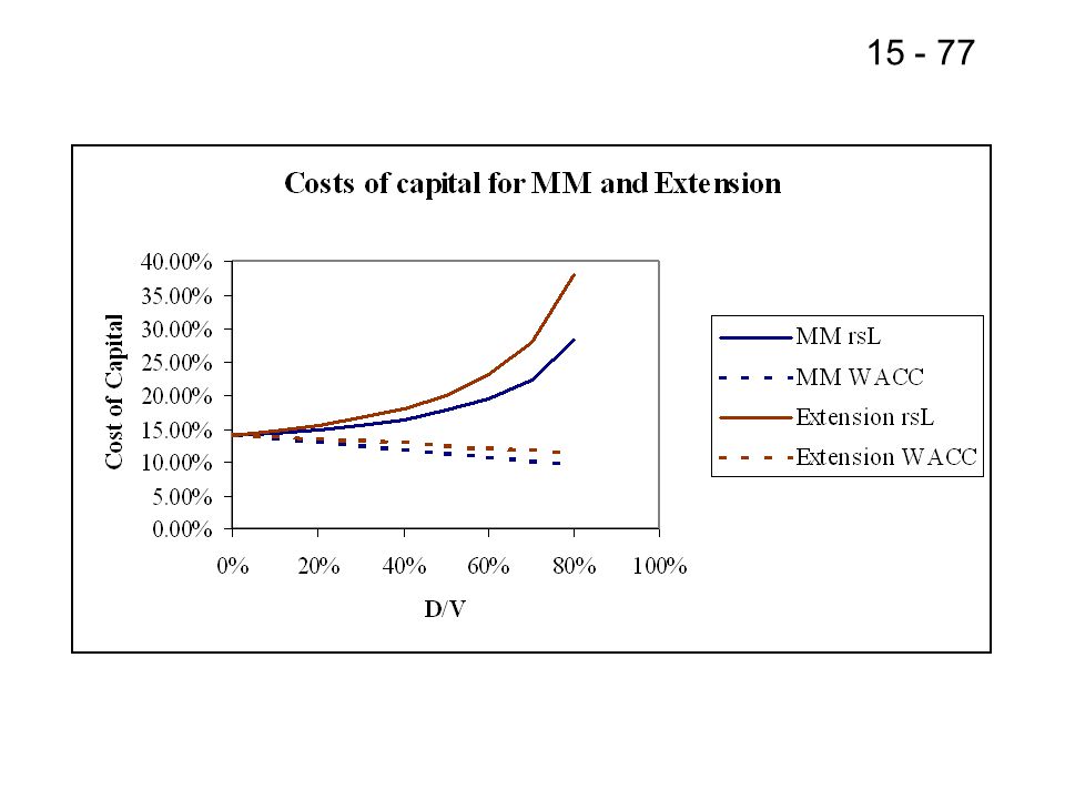
76 Cost of equity and WACC Just like with MM with taxes, the cost of equity increases with D/V, and the WACC declines. But since rsL doesn't have the (1-T) factor in it, for a given D/V, rsL is greater than MM would predict, and WACC is greater than MM would predict.

77

78 What if L's debt is risky? If L's debt is risky then, by definition, management might default on it. The decision to make a payment on the debt or to default looks very much like the decision whether to exercise a call option. So the equity looks like an option.

79 Equity as an option Suppose the firm has $2 million face value of 1-year zero coupon debt, and the current value of the firm (debt plus equity) is $4 million. If the firm pays off the debt when it matures, the equity holders get to keep the firm. If not, they get nothing because the debtholders foreclose.

80 Equity as an option The equity holder's position looks like a call option with P = underlying value of firm = $4 million X = exercise price = $2 million t = time to maturity = 1 year Suppose rRF = 6%  = volatility of debt + equity = 0.60

81 Use Black-Scholes to price this option
V = P[N(d1)] - Xe -rRFt[N(d2)]. d1 =  t d2 = d1 -  t. ln(P/X) + [rRF + (2/2)]t

82 Black-Scholes Solution
V = $4[N(d1)] - $2e-(0.06)(1.0)[N(d2)]. ln($4/$2) + [( /2)](1.0) (0.60)(1.0) = d2 = d1 - (0.60)(1.0) = d = = d1 =

83 = $2.196 Million = Value of Equity
N(d1) = N(1.5552) = N(d2) = N(0.9552) = Note: Values obtained from Excel using NORMSDIST function. V = $4(0.9401) - $2e-0.06(0.8303) = $ $2(0.9418)(0.8303) = $2.196 Million = Value of Equity

84 Value of Debt The value of debt must be what is left over: Value of debt = Total Value – Equity = $4 million – million = $1.804 million

85 This value of debt gives us a yield
Debt yield for 1-year zero coupon debt = (face value / price) – 1 = ($2 million/ million) – 1 = 10.9%

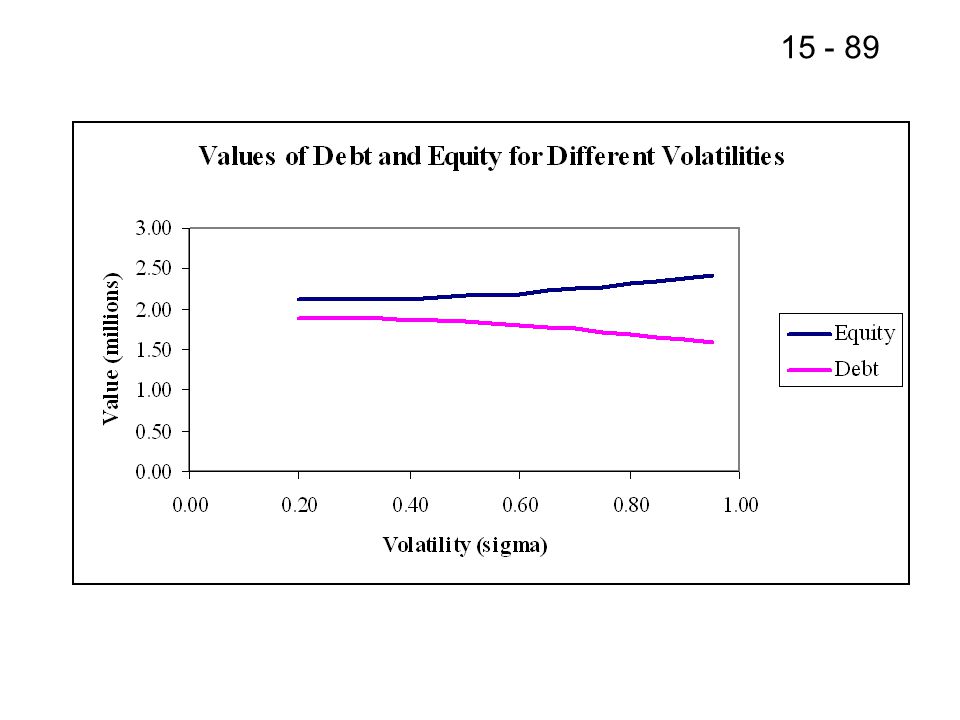
86 How does  affect an option's value?
Higher volatility  means higher option value.

87 Managerial Incentives
When an investor buys a stock option, the riskiness of the stock () is already determined. But a manager can change a firm's  by changing the assets the firm invests in. That means changing  can change the value of the equity, even if it doesn't change the expected cash flows:

88 Managerial Incentives
So changing  can transfer wealth from bondholders to stockholders by making the option value of the stock worth more, which makes what is left, the debt value, worth less.

89

90 Bait and Switch Managers who know this might tell debtholders they are going to invest in one kind of asset, and, instead, invest in riskier assets. This is called bait and switch and bondholders will require higher interest rates for firms that do this, or refuse to do business with them.

91 If the debt is risky coupon debt
If the risky debt has coupons, then with each coupon payment management has an option on an option—if it makes the interest payment then it purchases the right to later make the principal payment and keep the firm. This is called a compound option.