Pengantar Sistem Dinamik

Presentasi berjudul: "Pengantar Sistem Dinamik"— Transcript presentasi:

1 Pengantar Sistem Dinamik
Dr. Asep Sofyan Teknik Lingkungan ITB

2 Apakah Sistem Dinamik itu?
Sistem dinamik: Pemodelan dan simulasi komputer untuk mempelajari dan mengelola sistem umpan balik yang rumit (complex feedback systems), seperti bisnis, sistem lingkungan, sistem sosial, dsb. Sistem: Kumpulan elemen yang saling berinteraksi, berfungsi bersama untuk tujuan tertentu. Umpan balik menjadi sangat penting Masalah dinamik Mengandung jumlah (kuantitas) yang selalu bervariasi Variasi dapat dijelaskan dalam hubungan sebab akibat Hubungan sebab akibat dapat terjadi dalam sistem tertutup yang mengandung lingkaran umpan balik (feedback loops)

3 Sejarah Cybernetics (Wiener, 1948): studi yang mempelajari bagaimana sistem biologi, rekayasa, sosial, dan ekonomi dikendalikan dan diatur Industrial Dynamics (Forrester, 1961): mengaplikasikan prinsip “cybernetics” ke dalam sistem industri System Dynamics: karya Forrester semakin meluas meliputi sistem sosial dan ekonomi Dengan perkembangan komputer yang sangat cepat, Sistem Dinamik menyediakan kerangka kerja dalam menyelesaikan permasalahan sistem sosial dan ekonomi

4 Tahap Pemodelan Sistem Dinamik
Identifikasi masalah Membangun hipotesis dinamik yang menjelaskan hubungan sebab akibat dari masalah termaksud Membuat struktur dasar grafik sebab akibat Melengkapi grafik sebab akibat dengan informasi Mengubah grafik sebab akibat yang telah dilengkapi menjadi grafik alir Sistem Dinamik Menyalin grafik alir Sistem Dinamik kedalam program DYNAMO, Stella, Vensim, Powersim, atau persamaan matematika

5 Aspek penting Berfikir dalam terminologi hubungan sebab akibat
Fokus pada keterkaitan umpan balik (feedback linkages) diantara komponen- komponen sistem Membuat batasan sistem untuk menentukan komponen yang masuk dan tidak di dalam sistem

6 Hubungan Sebab Akibat Berfikir sebab akibat adalah kunci dalam mengorganisir ide-ide dalam studi Sistem Dinamik Gunakan kata `menyebabkan` atau `mempengaruhi` untuk menjelaskan hubungan antar komponen di dalam sistem Contoh yang logis (misalnya hukum fisika) makan berat bertambah api  asap Contoh yang tidak logis (sosiologi, ekonomi) Pakai sabuk pengaman  mengurangi korban fatal dalam kecelakaan lalu lintas

7 Umpan balik (Feedback)
Berfikir sebab akibat saja tidak cukup laut  evaporasi  awan  hujan  laut  … Umpan balik: untuk mengatur/ mengendalikan sistem, yaitu berupa suatu sebab yang terlibat dalam sistem namun dapat mempengaruhi dirinya sendiri Umpan balik sangat penting dalam studi Sistem Dinamik

8 Causal Loop Diagram (CLD)
CLD menunjukkan struktur umpan balik dari sistem Gaji VS Kinerja Gaji  Kinerja Kinerja  Gaji Lelah VS Tidur Lelah  tidur Tidur  lelah ?

9 Penanda CLD + : jika penyebab naik, akibat akan naik (pertumbuhan, penguatan), jika penyebab turun, akibat akan turun - : jika penyebab naik, akibat akan turun, jika penyebab turun, akibat akan naik + + + -

10 CLD dengan Positive Feedback Loop
Gaji  Kinerja, Kinerja  Gaji Semakin gaji naik Semakin baik kinerja + Semakin baik kinerja Gaji akan semakin naik + Semakin gaji naik Semakin baik kinerja +

11 CLD dng Negative Feedback Loop
Lelah  Tidur, Tidur  Lelah The more I sleep The less tired I am The less tired I am The less I sleep The more tired I am The more I sleep The less I sleep The more tired I am + - -

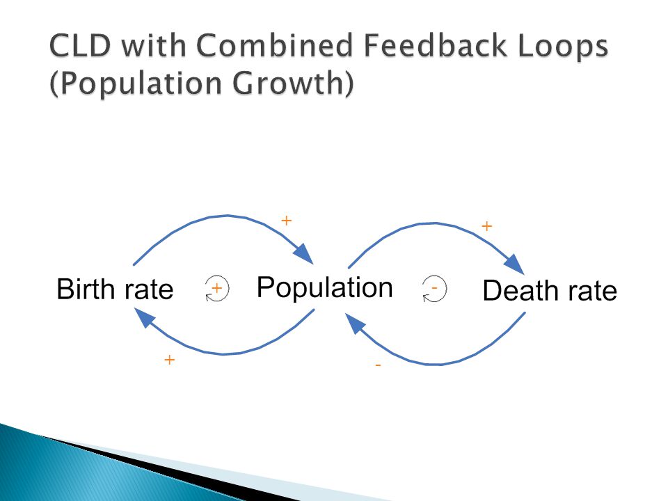
12 CLD with Combined Feedback Loops (Population Growth)
+ + + - + -

13 CLD with Nested Feedback Loops (Self-Regulating Biosphere)
Evaporation  clouds  rain  amount of water  evaporation  … + - + + - - + + + + - + +

14 Exogenous Items Items that affect other items in the system but are not themselves affected by anything in the system Arrows are drawn from these items but there are no arrows drawn to these items + - - +

15 Delays Systems often respond sluggishly (dgn malas)
From the example below, once the trees are planted, the harvest rate can be ‘0’ until the trees grow enough to harvest delay -

16 Loop Dominance There are systems which have more than one feedback loop within them A particular loop in a system of more than one loop is most responsible for the overall behavior of that system The dominating loop might shift over time When a feedback loop is within another, one loop must dominate Stable conditions will exist when negative loops dominate positive loops

17 Example

18 Flow Graph Symbols Level Rate Flow arc Auxiliary Cause-and-effect arc
Source/Sink Constant

19 Level: Stock, accumulation, or state variable
A quantity that accumulates over time Change its value by accumulating or integrating rates Change continuously over time even when the rates are changing discontinuously

20 Rate/Flow: Flow, activity, movement Change the values of levels
The value of a rate is Not dependent on previous values of that rate But dependent on the levels in a system along with exogenous influences

21 Auxiliary: Arise when the formulation of a level’s influence on a rate involves one or more intermediate calculations Often useful in formulating complex rate equations Used for ease of communication and clarity Value changes immediately in response to changes in levels or exogenous influences

22 Source and Sink: Source represents systems of levels and rates outside the boundary of the model Sink is where flows terminate outside the system

23 Example 1 (Population and birth)
Births Population

24 Example 2 (Children and adults)
- + Children maturing Births children Adults

25 average lifetime = 8 Units: Year birth rate = 0.125 Units: fraction/Year births = Population * birth rate Units: rabbit/Year deaths = Population / average lifetime Population = INTEG(births - deaths,1000) Units: rabbit

26 From Causal Loop Diagram To Simulation Models 1
Causal Graph Flow Graph R L Equations dL/dt = k1*R(t) R(t) = k2*L(t)  dL/dt = k1*k2*L(t) Block Model L’ L ∫ k1*k2

27 From Causal Loop Diagram To Simulation Models 2
Flow Graph Equations dL/dt = R1 – R2 R2 = k2*L R1 = k1  dL/dt = k1 - k2*L R1 R2 L Block Model L1’ L1 ∫ k2 k1 -

28 From Causal Loop Diagram To Simulation Models 3
Flow Graph Equations dL1/dt = R1 – R2 dL2/dt = R2 – R3 R1 = k1 R2 = K2 * L1 R3 = K3 * L2  dL1/dt = k1 – k2*L1  dL2/dt = k2*L1 – K3*L2 R1 R2 R3 L1 L2 Block Model L1’ L1 L2’ L2 ∫ - ∫ k2 k3 k1 -

29 Building construction
Problem statement Fixed area of available land for construction New buildings are constructed while old buildings are demolished Primary state variable will be the total number of buildings over time Causal Graph - - - -

30 Simulation models Flow Graph Equations dBl/dt = Cr – Dr
Cr = f1(CF, Bl) Dr = f2(AL,Bl) CF = f3(FLO) FLO = f4(LA,AA,Bl) Construction (C) Demolition (D) Industrial Buildings (B) Average lifetime for buildings (AL) Construction fraction (CF) Fraction of land occupied (FLO) Land available for industrial buildings (LA) Average area per building (AA)

31 References Simulation Model Design and Execution, Fishwick, Prentice-Hall, 1995 (Textbook) Introduction to Computer Simulation: A system dynamics modeling approach, Nancy Roberts et al, Addison-wesley, 1983 Business Dynamics: Systems thinking and modeling for a complex world, John D. Sterman, McGraw-Hill,2000