Modul-8 : Algoritma dan Struktur Data

Presentasi berjudul: "Modul-8 : Algoritma dan Struktur Data"— Transcript presentasi:

1 Modul-8 : Algoritma dan Struktur Data
Sorting Algorithms Modul-8 : Algoritma dan Struktur Data

2 Heap-Sort Binary heap digunakan sebagai struktur data dalam algoritma Heap-Sort Sebagaimana diketahui, ketika suatu Heap dibangun maka kunci utamanya adalah: node atas selalu mengandung elemen lebih besar dari kedua node dibawahnya Apabila elemen berikutnya ternyata lebih besar dari elemen root, maka harus di “swap” dan lakukan: proses “heapify” lagi Root dari suatu Heap sort mengandung elemen terbesar dari semua elemen dalam Heap

3 Proses Heap-Sort dapat dijelaskan sbb:
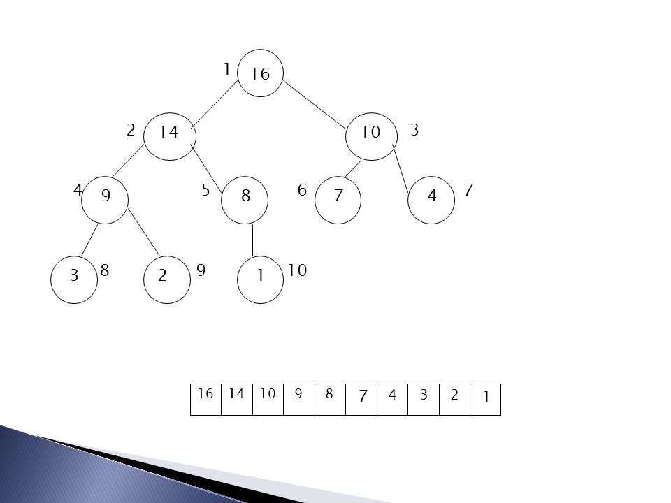
Representasikan Heap dengan n elemen dalam sebuah array A[n] Elemen root tempatkan pada A[1] Elemen A[2i] adalah node kiri dibawah A[i] Elemen A[2i+1] adalah node kanan dibawah A[i] Contoh: array A=[ ] mewakili binary-heap sbb: Ambil nilai root (terbesar) A[1..n-1] dan pertukarkan dengan elemen terakhir dalam array, A[n] Bentuk Heap dari (n-1) elemen, dari A[1] hingga A[n-1] Ulangi langkah 6 dimana indeks terakhir berkurang setiap langkah.

4 1 14 10 8 7 9 3 2 4 16 16

5 1 14 10 9 8 7 4 3 2 16 16

6 MAX-HEAPIFY(A, i) 1 l ← LEFT(i) 2 r ← RIGHT(i) 3 if l ≤ heap-size[A] and A[l] > A[i] 4 then largest ← l 5 else largest ← i 6 if r ≤ heap-size[A] and A[r] > A[largest] then largest ← r 8 if largest ≠ i 9 then exchange A[i] ↔ A[largest] MAX-HEAPIFY(A, largest)

7 BUILD-MAX-HEAP(A) 1 heap-size[A] ← length[A] 2 for i ← ⌊length[A]/2⌋ downto 1 3 do MAX-HEAPIFY(A, i)

8

9 HEAPSORT(A) 1 BUILD-MAX-HEAP(A) 2 for i ← length[A] downto 2 do exchange A[1] ↔ A[i] heap-size[A] ← heap-size[A] - 1 MAX-HEAPIFY(A, 1)

10

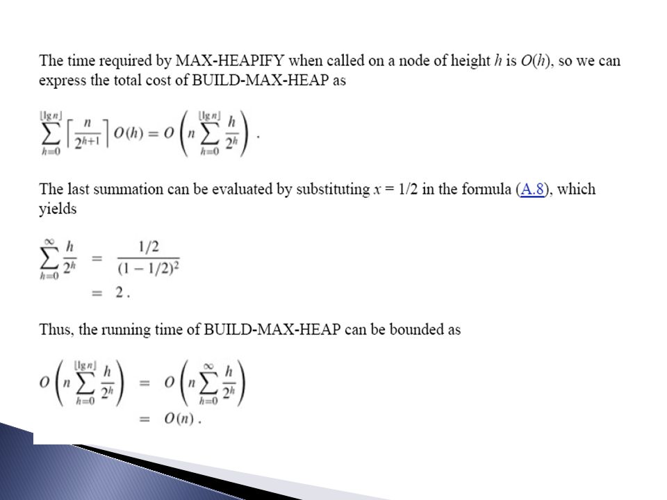
11 Analisis: Prosedur Heapify(i,j) adalah pembentukan binary heap dengan kompleksitas O(log n) Kemudian prosedur ini dipanggil n kali (Build-Max- Heap) sehingga secara keseluruhan kompleksitas adalah O(n log n)

12 Quick-Sort Quick-sort adalah teknik pengurutan data yang memiliki kerumitan rata-rata O(n log n) tetapi dalam “worst-case” bisa mencapai O(n2) Teknik Quick-sort berbasis teknik divide- and-conquer, sbb: Divide : array A[p..r] dibagi menjadi A[p..q] dan A[q+1 ..r] sehingga setiap elemen A[p..q] lebih kecil dari atau sama dengan setiap elemen A[q+1..r] Conquer : subarray A[p..q] dan A[q+1..r] juga di- sort menurut Quick-Sort Combine : pada akhirnya A[p..r] akan ber-urutan

13 QuickSort(A,p,r) if (p < r) then q  Partisi(A,p,r); QuickSort(A,p,q); QuickSort(A,q+1,r); Partisi(A,p,r) x  A[p]; i  (p-1); j  (r+1); while (true) { repeat (j j -1) until (A[j] <= x) repeat (i  i+1) until (A[i] >= x) if (i < j) then Swap(A[i], A[j]) else Return (j) }

14 Analisis: Worst-case : terjadi apabila partisi memberikan q=(n-1), atau subarray pertama = A[1..n-1] dan subarray kedua hanya 1 elemen A[n] T(n) = T(n-1) + (n), jadi T(1) = (1) Solusinya = Average-case : karena mengikuti divide-and- conquer maka: T(n) = 2 T(n/2) + (n) sehingga solusi-nya adalah O(n log n)

15 Radix Sort Radix sort biasa digunakan pada basis data yang akan di-urutkan melalui kunci yang berantai, misalnya akan diurutkan menurut tanggal lahir, maka harus dilakukan sort 3 langkah, pertama menurut tahun, kemudian menurut bulan, dan terakhir menurut tanggal Pada sortir angka, maka radix sort diterapkan pada setiap digit RADIX-SORT(A, d) 1 for i ← 1 to d 2 do use a stable sort to sort array A on digit i Suarga

16 The analysis of the running time depends on the stable sort used as the intermediate sorting algorithm. When each digit is in the range 0 to k-1 (so that it can take on k possible values), and k is not too large, counting sort is the obvious choice. Each pass over n d-digit numbers then takes time Θ(n + k). There are d passes, so the total time for radix sort is Θ(d(n + k)). Suarga

17 Counting Sort Counting sort assumes that each of the n input elements is an integer in the range 0 to k, for some integer k. When k = O(n), the sort runs in Θ(n) time. In the code for counting sort, we assume that the input is an array A[1 n], and thus length[A] = n. We require two other arrays: the array B[1 n] holds the sorted output, and the array C[0 k] provides temporary working storage. Suarga

18 5 ▹ C[i] now contains the number of elements equal to i.
COUNTING-SORT(A, B, k) 1 for i ← 0 to k 2 do C[i] ← 0 3 for j ← 1 to length[A] 4 do C[A[j]] ← C[A[j]] + 1 5 ▹ C[i] now contains the number of elements equal to i. 6 for i ← 1 to k 7 do C[i] ← C[i] + C[i - 1] 8 ▹ C[i] now contains the number of elements less than or equal to i. 9 for j ← length[A] downto 1 10 do B[C[A[j]]] ← A[j] C[A[j]] ← C[A[j]] - 1 Suarga

19 The operation of COUNTING-SORT on an input array A[1 8], where each
element of A is a nonnegative integer no larger than k = 5. (a) The array A and the auxiliary array C after line 4. (b) The array C after line 7. (c)-(e) The output array B and the auxiliary array C after one, two, and three iterations of the loop in lines 9-11, respectively. Only the lightly shaded elements of array B have been filled in. (f) The final sorted output array B. Suarga

20 How much time does counting sort require
How much time does counting sort require? The for loop of lines 1-2 takes time Θ(k), the for loop of lines 3-4 takes time Θ(n), the for loop of lines 6-7 takes time Θ(k), and the for loop of lines 9-11 takes time Θ(n). Thus, the overall time is Θ(k+n). In practice, we usually use counting sort when we have k = O(n), in which case the running time is Θ(n). Suarga

21 Bucket Sort Bucket sort runs in linear time when the input is drawn from a uniform distribution. Like counting sort, bucket sort is fast because it assumes something about the input. bucket sort assumes that the input is generated by a random process that distributes elements uniformly over the interval [0, 1). Suarga

22 The idea of bucket sort is to divide the interval [0, 1) into n equal-sized subintervals, or buckets, and then distribute the n input numbers into the buckets. Our code for bucket sort assumes that the input is an n-element array A and that each element A[i] in the array satisfies 0 ≤ A[i] < 1. The code requires an auxiliary array B[0 n - 1] of linked lists (buckets) and assumes that there is a mechanism for maintaining such lists. Suarga

23 BUCKET-SORT(A) 1 n ← length[A] 2 for i ← 1 to n 3 do insert A[i] into list B[⌊n A[i]⌋] 4 for i ← 0 to n do sort list B[i] with insertion sort 6 concatenate the lists B[0], B[1], . . ., B[n - 1] together in order Suarga

24 The operation of BUCKET-SORT. (a) The input array A[1 10]
The operation of BUCKET-SORT. (a) The input array A[1 10]. (b) The array B[0 9] of sorted lists (buckets) after line 5 of the algorithm. Bucket i holds values in the half-open interval [i/10, (i + 1)/10). The sorted output consists of a concatenation in order of the lists B[0], B[1], . . ., B[9]. Suarga

25 the running time of bucket sort is
we conclude that the expected time for bucket sort is Θ(n) + n · O(2 - 1/n) = Θ(n). Suarga