Grafika Komputer dan Visualisasi Disusun oleh : Silvester Dian Handy Permana, S.T., M.T.I. Fakultas Telematika, Universitas Trilogi Pertemuan 15 : Kurva.

Presentasi berjudul: "Grafika Komputer dan Visualisasi Disusun oleh : Silvester Dian Handy Permana, S.T., M.T.I. Fakultas Telematika, Universitas Trilogi Pertemuan 15 : Kurva."— Transcript presentasi:

1 Grafika Komputer dan Visualisasi Disusun oleh : Silvester Dian Handy Permana, S.T., M.T.I. Fakultas Telematika, Universitas Trilogi Pertemuan 15 : Kurva Bezier

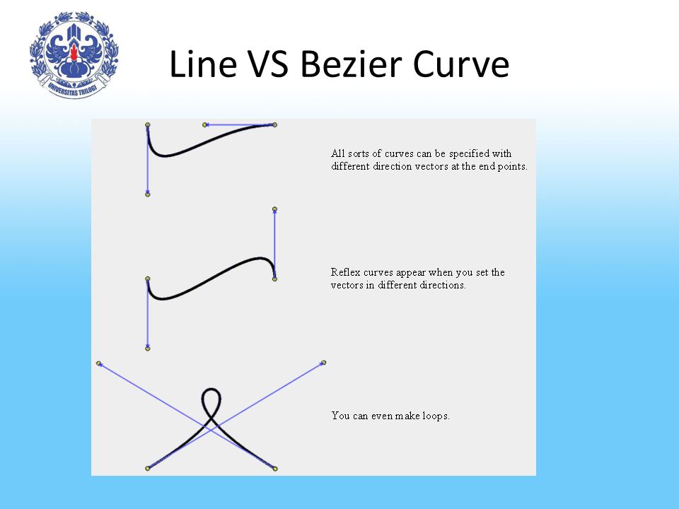
2 Line VS Bezier Curve

3

4 Drawing the Curve:

5

6 Algoritma de Casteljau Algoritma untuk membuat kurva menggunakan sejumlah titik kontrol, dan menggunakan teknik in-betweening untuk mendapatkan kurva yang diinginkan. Dikembangkan oleh P. de Casteljau, dan merupakan cikal bakal kurva Bezier, yang secara terpisah dikembangkan lebih lanjut oleh P. Bezier.

7 Algoritma de Casteljau Implementasi Algoritma de Casteljau yang paling sederhana adalah pembentukan kurva berdasarkan 3 titik kontrol yaitu

8 Representasi de Casteljau Dengan memilih nilai t antara 0 dan 1, tentukan titik P 0 1 sepanjang t bagian dari P o ke P 1. Dengan cara yang sama, tentukan titik titik P 1 1 sepanjang t bagian dari P 1 ke P 2, sehingga titik- titik tersebut dapat dinyatakan sebagai berikut: P 0 1 (t) = (1-t) P 0 + t.P 1 P 1 1 (t) = (1-t) P 1 + t.P 2

9 Representasi de Casteljau Dengan menggunakan interpolasi linear yang sama, bisa ditentukan titik P 0 2 sepanjang t bagian dari P 0 1 ke P 1 1, yaitu : P 0 2 (t) = (1-t) P 0 1 (t) + t.P 1 1 (t) P 0 2 (t) = (1-t) 2 P 0 + 2t.(1-t).P 1 + t 2.P 2 Persamaan di atas adalah persamaan parabola, sehingga kurva yang terbentuk pada gambar di atas tidak lain adalah suatu parabola.

10 Representasi de Casteljau Dengan menggunakan asumsi yang sama, oleh de Casteljau persamaan di atas dikembangkan untuk membentuk sembarang kurva dengan menggunakan (N+1) buah titik kontrol. Untuk suatu nilat t tertentu, kita bisa membuat "generasi" ke r dalam proses in-between berdasar hasil generasi ke (r-1), yaitu : P i r (t) = (1-t)P i r-1 (t) + t.P i+1 r-1 (t). untuk setiap generasi, r=1,2,...,N dan untuk i = 0,1,…,N-r Proses dimulai dari P i untuk P i 0 Generasi "terakhir.' dari persamaan di atas, P 0 N (t), disebut dengan Kurva Bezier.

11 Kurva Bezier Kurva Bezier digunakan dalam komputer grafis untuk menghasilkan kurva yang cukup mulus di semua skala (berbeda denga garis poligonal). Kurva Bezier diberi nama setelah penemu mereka, Dr. Pierre Bezier. Bezier adalah seorang insinyur dengan perusahaan mobil Renault dan ditetapkan dalam awal 1960-an untuk mengembangkan formulasi kurva yang digunakan untuk desain. Kurva adalah fungsi parametrik empat poin; dua titik akhir dan dua "kontrol" poin. Kurva menghubungkan titik akhir, tapi tidak selalu menyentuhtitik kontrol. Persamaan Bezier bentuk umum, yang menjelaskan setiap titik pada kurva sebagai fungsi waktu

12 Kurva Bezier

13

14 Kurva bezier Perhitungan bezier bisa dibantu dengan cara sebagai berikut : Untuk n titik kontrol maka persamaan kurva bezier adalah (x+y)n-1 Ganti x dengan (1-t) dan y dengan t, kemudian selesaikan persamaan dengan titik yang dimaksud

15 Contoh soal Diketahui 3 buah titik kontrol dengan koordinat C1(1,2), C2(7,10), C3(15,4), dengan menggunakan kenaikan t=0.02 maka tentukanlah: 1. Berapa titik yang digunakan untuk membangun kurva bezier? 2. Berapa nilai titik pada kurva pada saat t=0.8?

16 solusi

17 2.Karena terdiri dari 3 titik kontrol maka persamaan menjadi : (x+y) 3-1 = (x+y) 2 x 2 + 2xy + y 2 = 0 x = (1-t) dan y = t Maka persamaan tersebut menjadi : L(t) = (1-t) 2 + 2(1-t) t + t 2

18 solusi 2.Titik untuk t = 0.8 x = (1-t) 2.x1 + 2(1-t)t.x 2 + t 2.x3 y = (1-t) 2.y1 + 2(1-t)t.y2 + t 2.y3 Catatan : x1, x2, x3, y1, y2 dan y3 diambil dari titik kontrol x = (1-0.8) 2.1 + 2(1-0.8)(0.8).7 + (0.8) 2.15 x = 0.04 + 2.24 + 9.6 = 11.88 ~ 12 y = (1-0.8) 2.2 + 2(1-0.8)(0.8).10 + (0.8) 2.4 y = 0.08 + 3.2 + 2.56 = 5.84 ~ 6 Nilai titik pada kurva saat t = 0.8 adalah (12,6)

19 Soal (untuk 4 titik kontrol) Diketahui 4 buah titik kontrol dengan koordinat C1(0,1), C2(1,2), C3(2,2), C4(3,1) dengan menggunakan kenaikan t=0.02 maka tentukanlah: Berapa nilai titik pada kurva pada saat t=0.8?

20 Ilustrasi Pembuatan Kurva Bezier

21 Linear Bézier curves Given points P 0 and P 1, a linear Bézier curve is simply a straight line between those two points. The curve is given by and is equivalent to linear interpolation.

22 Ilustrasi: kurva linier The t in the function for a linear Bézier curve can be thought of as describing how far B(t) is from P 0 to P 1. For example when t=0.25, B(t) is one quarter of the way from point P 0 to P 1. As t varies from 0 to 1, B(t) describes a curved line from P 0 to P 1.

23 Ilustrasi: kurva linier

24 Quadratic Bézier curves A quadratic Bézier curve is the path traced by the function B(t), given points P 0, P 1, and P 2, A quadratic Bézier curve is also a parabolic segment.

25 Ilustrasi: kurva kuadratik For quadratic Bézier curves one can construct intermediate points Q 0 and Q 1 such that as t varies from 0 to 1: Point Q 0 (t) varies from P 0 to P 1 and describes a linear Bézier curve. Point Q 1 (t) varies from P 1 to P 2 and describes a linear Bézier curve. Point B(t) is interpolated linearly between Q 0 (t) to Q 1 (t) and describes a quadratic Bézier curve.

26 Ilustrasi: kurva kuadratik

27 Cubic Bézier curves Four points P 0, P 1, P 2 and P 3 in the plane or in higher-dimensional space define a cubic Bézier curve. The curve starts at P 0 going toward P 1 and arrives at P 3 coming from the direction of P 2. Usually, it will not pass through P 1 or P 2 ; these points are only there to provide directional information. The distance between P 0 and P 1 determines "how far" and "how fast" the curve moves towards P 1 before turning towards P 2.

28 Ilustrasi : Kurva Cubic For higher-order curves one needs correspondingly more intermediate points. For cubic curves one can construct intermediate points Q 0, Q 1, and Q 2 that describe linear Bézier curves, and points R 0 & R 1 that describe quadratic Bézier curves:

29 Ilustrasi : Kurva Cubic

30 For fourth-order curves one can construct intermediate points Q 0, Q 1, Q 2 & Q 3 that describe linear Bézier curves, points R 0,R 1 & R 2 that describe quadratic Bézier curves, and points S 0 & S 1 that describe cubic Bézier curves:

31 Ilustrasi : Kurva Cubic

32 For fifth-order curves, one can construct similar intermediate points.

33 The Math Behind the Bezier Curve

34 A cubic Bezier curve is defined by four points. Two are endpoints. (x 0,y 0 ) is the origin endpoint. (x 3,y 3 ) is the destination endpoint. The points (x 1,y 1 ) and (x 2,y 2 ) are control points.

35 Two equations define the points on the curve. Both are evaluated for an arbitrary number of values of t between 0 and 1. One equation yields values for x, the other yields values for y. As increasing values for t are supplied to the equations, the point defined by x(t),y(t)moves from the origin to the destination The Math Behind the Bezier Curve

36 This is how the equations are defined in Adobe's PostScript references. x(t) = a x t 3 + b x t 2 + c x t + x 0 x 1 = x 0 + c x / 3 x 2 = x 1 + (c x + b x ) / 3 x 3 = x 0 + c x + b x + a x y(t) = a y t 3 + b y t 2 + c y t + y 0 y 1 = y 0 + c y / 3 y 2 = y 1 + (c y + b y ) / 3 y 3 = y 0 + c y + b y + a y The Math Behind the Bezier Curve

37 This method of definition can be reverse- engineered so that it'll give up the coefficient values based on the points described above: c x = 3 (x 1 - x 0 ) b x = 3 (x 2 - x 1 ) - c x a x = x 3 - x 0 - c x - b x c y = 3 (y 1 - y 0 ) b y = 3 (y 2 - y 1 ) - c y a y = y 3 - y 0 - c y - b y The Math Behind the Bezier Curve

38 QA