Production Planning / Agregat Planning

Presentasi berjudul: "Production Planning / Agregat Planning"— Transcript presentasi:

1 Production Planning / Agregat Planning
M A C H F U D

2 Production Planning: Units of Measure
Entire Product Line Long-Range Capacity Planning Aggregate Planning Product Family Specific Product Model Master Production Scheduling Production Planning and Control Systems Labor, Materials, Machines Pond Draining Systems Push Systems Pull Systems Focusing on Bottlenecks

3 Long-term Intermediate-term Intermediate-term Short-term
Capacity Planning, Aggregate Planning, Master Schedule, and Short-Term Scheduling Capacity Planning 1. Facility Size 2. Equipment Procurement Long-term Aggregate Planning 1. Facility Utilization 2. Personnel needs 3. Subcontracting Intermediate-term Master Schedule 1. MRP 2. Disaggregation of master plan Intermediate-term Short-term Scheduling 1. Work center loading 2. Job sequencing Short-term

4 Hierarchical Production Planning
Allocates production among plants Determines seasonal plan by product type Determines monthly item production schedules Decision Process Decision Level Corporate Plant manager Shop superintendent Annual demand by item and by region Monthly demand for 15 months by product type for 5 months by item Forecasts needed 5 5

5 Relationships Between OM Elements
Marketplace and Demand Research and Technology Work Force Product Decisions Raw Materials Available Inventory On Hand Process Planning & Decisions External Capacity Plant Demand Forecasts, orders Aggregate Plan for Production Master Production Schedule Detailed Work Schedules Priority Planning & Scheduling

6 Aggregate Planning

7 Mengapa Perencanaan Agregat Perlu
Pembebanan fasilitas secara penuh dan meminimumkan overloading dan underloading Menjamin tersedianya kapasitas yang cukup untuk memenuhi expected demand Merencanakan perubahan tingkat produksi secara teratur dan sistematik untuk memenuhi fluktuasi permintaan (the peaks and valleys of expected customer demand) Memperoleh output terbesar dengan sumberdaya produksi yang tersedia / terbatas.

8 Inputs Hasil prakiraan permintaan secara agregat dalam horizon perencanaan tertentu (6-18 bulan) Alternatif kebijakan untuk penyesuaian kapasitas jangka pendek ke kapasitas jangka menengah, dan dampak setiap alternatif terhadap kapasitas dan biaya Status sistem produksi saat ini, yaitu jumlah tenaga kerja, tingkat persediaan, dan tingkat produksi.

9 Outputs Suatu Rencana Produksi: keputusan secara agregat tentang
Jumlah tenaga kerja (workforce level) Tingkat persediaan Tingkat produksi secara agregat pada setiap periode dalam horizon perencanaan.  Total biaya produksi yang “terbaik” selama horizon perencanaan. Proyeksi biaya jika rencana produksi dilaksanakan.

10 Penyesuaian Kapasitas dalam horizon Medium
Jumlah tenaga kerja Hire or layoff full-time workers Hire or layoff part-time workers Hire or layoff contract workers Pendayagunaan tenaga kerja Overtime Idle time (undertime) Reduce hours worked Jumlah persediaan Finished goods inventory Backorders/lost sales Subcontract

11 Approaches Informal or Trial-and-Error Approach (Graphical Method)
Mathematically Optimal Approaches Linear Programming Linear Decision Rules Computer Search Heuristics

12 Comparison of Aggregate Planning Methods
Advantages Limitations Graphical Sederhana, mudah digunakan dan dipahami Banyak solusi; dan tidak optimal Linear Programming Memberikan solusi optimal Analisis sensitifitas dan dual memberikan informasi yang berguna. Kendala dapat segera dimasukkan Fungsi matematis: harus linear, bersifat deterministik, menggunakan asumsi yang tidak terlalu realistis. 12

13 Perbandingan antar Aggregate Planning Methods
Advantages Limitations Linear Decision Rules Memberikan solusi optimal Dapat untuk permintaan yang bersifat non-deterministic Menggunakan beberapa komponen biaya yang non-standard Membutuhkan Skilled personal Model Quadratic tidak selalu realistik. Tidak menjamin solusi yang optimal. Management Coefficients Model Sederhana, mudah digunakan dan dipahami. Merupakan upaya untuk menduplikasi proses pengambilan keputusan manager. Mudah diterapkan. Solusi tidak optimal. Berasumsi bahwa keputusan yg diambil pada masa lalu adalah baik. Model dibangun atas dasar “individual” dan bisa tidak sahih. (individual’s invalidate model) 12

14 Perbandingan antar Aggregate Planning Methods
Advantages Limitations Simulation Tidak ada batasan pada fungsi biaya tertentu atau struktur matematis. Dapat menguji berbagai keterkaitan atau hubungan. Tidak menjamin solusi yang optimal. Seringkali merupakan proses yang panjang dan mahal. 12

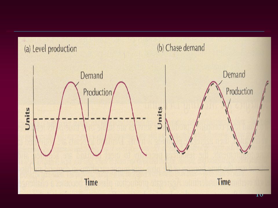
15 Pure Strategies for the Informal Approach
Matching Demand (Chase Strategy) Level Capacity (Level Strategy) Penyanggaan dengan persediaan (Buffering with inventory) Penyanggaan dengan mekanisme backlog (Buffering with backlog) Penyanggaan dengan mekanisme lembur dan subkontrak (Buffering with overtime or subcontracting)

16

17 Matching Demand Strategy (Chase strategy)
Kapasitas (produksi) pada setiap periode persis sama dengan forecasted aggregate demand Variasi kapasitas (produksi) dilakukan dengan memvariasikan jumlah tenaga kerja. Persediaan produk akhir – minimal. Biaya tenaga kerja dan bahan cenderung tinggi, karena intensitas perubahan yang tinggi.

18 Mengembangkan dan Mengevaluasi Chase Production Plan
Tingkat produksi ditentukan atas dasar the forecasted aggregate demand The forecasted aggregate demand dikonevrsi ke jumlah jumlah tenaga kerja yang dibutuhkan dengan menggunakan informasi waktu baku produksi. Biaya utama dari strategi ini adalah biaya akibat perubahan jumlah tenaga kerja dari waktu ke waktu, dalam hal ini biaya hirings dan layoffs

19 Level Capacity Strategy
Kapasitas (tingkat produksi) dipertahankan tetap (konstan) selama horizon perencanaan. Selisih antara tingkat produksi yang konstan dan tingkat permintaan di sangga (buffered) dengan inventory, backlog, overtime, part-time labor and/or subcontracting

20 Mengembangkan dan Mengevaluasi the Level Production Plan
Menetapkan jumlah produksi yang tetap setiap periode, tanpa dilakukan perubahan jumlah tenaga kerja. Selisih antara jumlah produksi yang direncanakan dan prakiraan permintaan dipenuhi dengan persediaan atau dengan backorders, dalam hal ini tidak ada atau tidak dilakukan overtime, idle time, dan subcontracting . . . more

21 Mengembangkan dan Mengevaluasi the Level Production Plan
Biaya utama dari strategi ini adalah biaya menahan (kelebihan) persediaan dan biaya kekurangan persediaan (inventory carrying and backlogging costs) Tingkat persediaan (lebih atau kurang) pada akhir periode ditentukan dengan formula inventory balance equation: EIt = EIt-1 + (Pt - Dt )

22 Rencana Aggregate untuk Jasa
Untuk produk Jasa yang standardized, perencanaan aggregate lebih sederhana dibandingkan dengan sistem produksi yang memproduksi customized services Untuk customized services, Terdapat kesulitan dalam menentukan sifat dan spesifikasi operasi yang harus dilaksanakan untuk setiap pelanggan. Pelanggan dapat merupakan bagian integral dari sistem produksi. Jasa bersifat intangible (tidak fisik) sehingga tidak ada “istilah” finished-goods inventories yang dapat digunakan sebagai buffer antara kapasitas dan permintaan.

23 Preemptive Tactics There may be ways to manage the extremes of demand:
Discount prices during the valleys.... have a sale Peak-load pricing during the highs .... electric utilities, Nucor

24 Advantages/Disadvantages
Option Advantage Disadvantage Some Comments Changing inventory levels Changes in human resources are gradual, not abrupt production changes Inventory holding costs; Shortages may result in lost sales Applies mainly to production, not service, operations Varying workforce size by hiring or layoffs Avoids use of other alternatives Hiring, layoff, and training costs Used where size of labor pool is large

25 Advantages/Disadvantages - Continued
Option Advantage Disadvantage Some Comments Varying production rates through overtime or idle time Matches seasonal fluctuations without hiring/training costs Overtime premiums, tired workers, may not meet demand Allows flexibility within the aggregate plan Subcontracting Permits flexibility and smoothing of the firm's output Loss of quality control; reduced profits; loss of future business Applies mainly in production settings

26 Advantages/Disadvantages - Continued
Option Advantage Disadvantage Some Comments Using part-time Less costly and High Good for workers more flexible turnover/training unskilled jobs in than full-time costs; quality areas with large workers suffers; temporary labor scheduling pools difficult Influencing Tries to use Uncertainty in Creates demand excess capacity. demand. Hard to marketing ideas. Discounts draw match demand to Overbooking new customers. supply exactly. used in some businesses.

27 Advantage/Disadvantage - Continued
Option Advantage Disadvantage Some Comments Back ordering during high- demand periods May avoid overtime. Keeps capacity constant Customer must be willing to wait, but goodwill is lost. Many companies backorder. Counterseasonal products and service mixing Fully utilizes resources; allows stable workforce. May require skills or equipment outside a firm's areas of expertise. Risky finding products or services with opposite demand patterns.

28 Kasus Perencanaan Agregat
Suatu industri memproduksi beragam Candy. Berdasarkan hasil prakiraan dalam periode triwulan pada tahun yang akan datang adalah sbb: Kuartal 1 : unit Kuartal 2 : unit Kuartal 3 : unit Kuartal 4 : unit Tingkat produksi ditentukan oleh jumlah tenaga kerja, yang mana setiap pekerja mampu memproduksi 1000 unit per kuartal. Jumlah tenaga kerja pada awal perencanaan: 100 orang. Untuk meningkatkan kapasitas produksi perusahaan dapat menambah tanaga kerja dengan biaya $ 100 per orang, dan jika menurunkan kapasitas produksi, perusahaan dapat mem PHK dengan konsekuensi biaya $ 500 per orang. Perusahaan mengambil kebijakan tidak boleh terjadi kekurangan stok produk, apabila terjadi kelebihan stok biaya menahan persediaan: $ 0,50 per unit per kuartal. ? Apakah perusahaan mengambil skenario Level Startegy atau Chase Strategy dalam menentukan rencana produksi pada tahun yang akan datang.

29 Skenario Level Strategy
Terdapat beberapa alternatif dalam menentukan tingkat produksi yang tetap setiap kuartal: Berdasarkan kapasitas produksi (jumlah pekerja) yang ada. Berdasarkan rata-rata permintaan selama 4 kuartal. Yang penting harus memenuhi kendala bahwa setiap kuartal tidak boleh terjadi kekurangan produk, yang dapat dicek dengan menggunakan kurva kumulatif produksi dan kumulatif demand.. Jika digunakan alternatif rata-rata permintaan  tingkat produksi per kuartal : unit

30 Kumulatif produksi di atas kumulatif demand (atau garis kumulatif demand dan produksi tidal berpotongan)  tidak terjadi kekurangan stok

31 Aplikasi Linear Programming
Variabel keputusan: Jumlah Tenaga kerja  Jumlah Produksi  Jumlah yg direkrut / PHK Jumlah Inventory Tujuan Minimasi Total Biaya = Biaya Tenaga kerja + Biaya Inventory. Minimasi Z = 100 (H1+H2+H3+H4) (F1+F2+F3+F4) + 0,50 (I1+I2+I3+I4) dengan kendala

32 Kendala permintaan: It = It-1 + Pt – Dt t=1  P1 – I1 + Io = t=2  P2 – I2 + I1 = t=3  P3 – I3 + I2 = t=4  P4 – I4 + I3 = Kendala Produksi  Pt = 1000 Wt Kendala Tenaga Kerja: Wt =Wt-1 + Ht - Ft t=1  W1 + F1– H1 - Wo = 0. t=2  W2 + F2 – H2 - W1 = 0. t=3  W3 + F3 – H3 – W2= 0 t=4  W4 + F4 – H4 – W4= 0

33 Solusi Optimal P1 = 80  W1=80F1=20 & H1=0I1=0
Total Biaya $32.000,-

34 Aggregate Planning Example
A small manufacturing company with 200 employees produces umbrellas. The company produces the following three product lines: 1) the Executive Line, 2) the Durable Line and 3) the Compact line, as shown in the below Compact Line Executive Line Durable Line 8 8

35 Aggregate Planning Example: Demand for Executive Umbrellas
Number of working days: Jan: 22 Feb: 19 Mar: 21 Apr: 21 May: 22 Jun: 20 9 9

36 Aggregate Planning Example: Cost Information for Executive Umbrellas
11 11

37 Aggregate Planning Example: Determining Straight Labor Costs and Output for Executive Umbrellas
January = 22 [days/month] * 7.25 [productive hrs/worker] = [hrs/worker/month] / .15 [hrs/unit] $1,408 = 8 [$/hr] * 8 [paid hrs/day] * 22 [days/month] 11 11

38 Aggregate Planning Example: Determining Straight Labor Costs and Output for Executive Umbrellas
11 11

39 Aggregate Planning Example Chase Strategy for Executive Umbrellas
Objective: Adjust workforce level so as to eliminate the need to carry inventory from period to period 4,500 units is the demand in January (any combination of firm orders and forecast 250 is the starting inventory position 4,250 = 4,500 – 250 3.997 = 4,250 / 1,063.33 7 = workforce level at the beginning of January 3 = 7 – 4 = workers fired 4 = workforce level at end of January 0 = ending inventory level 13 13

40 Aggregate Planning Example Chase Strategy for Executive Umbrellas
13 13

41 Aggregate Planning Example Chase Strategy for Executive Umbrellas
January costs: $21, = 4,250 [units] * $5 [$/unit] $ 5, = [workers] * 1,408 [$/worker] $ = 3 [workers fired] * 250 [$/worker fired] 13 13

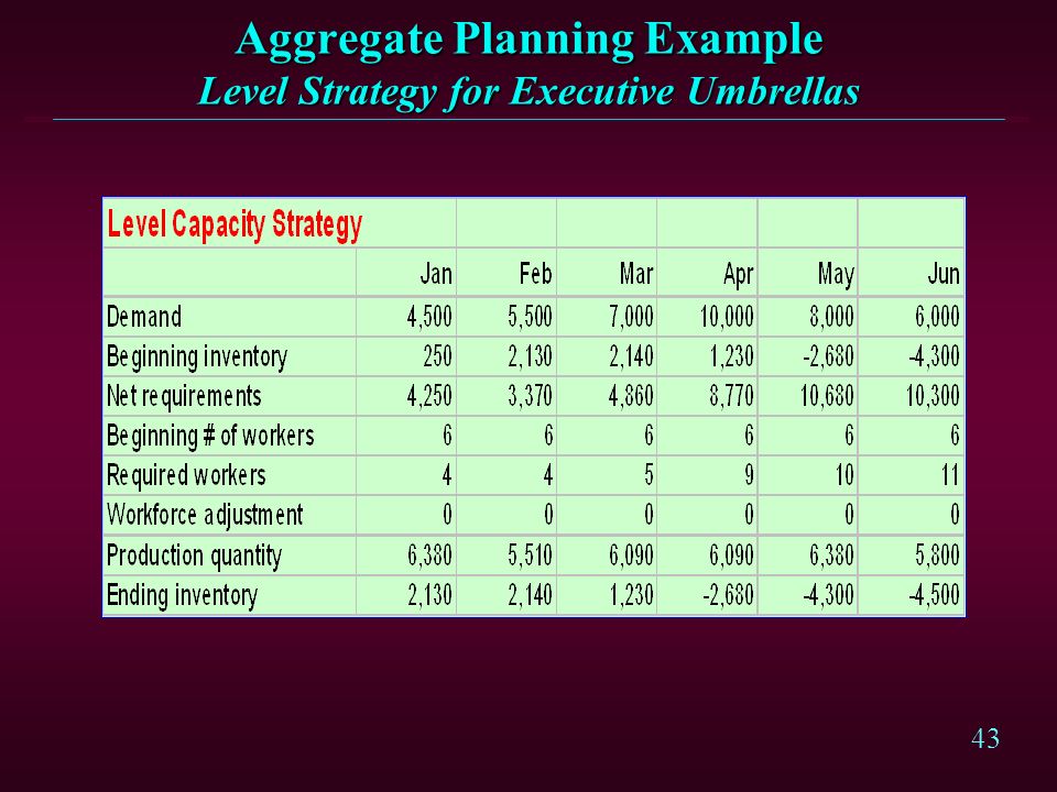
42 Aggregate Planning Example Level Strategy for Executive Umbrellas
Objective: Mengatur jumlah inventory sehingga menghilangkan perubahan jumlah tenaga kerja (tidak perlu hire dan fire dari periode ke periode) Assume that January is started with 6 employees 6,380 = 6 [employees] * 1, [units/worker] 2,130 = 6,380 – 4,250 (surplus) 16 16

43 Aggregate Planning Example Level Strategy for Executive Umbrellas
16 16

44 Aggregate Planning Example Level Strategy for Executive Umbrellas
January costs: $8,448 = 6 [workers] * $1,408 [$/worker] $ 31,900 = 6,380 [units] * $5 [$/unit] $ 2,130 = 2,130 [surplus units] * $1 [$/unit held/month] 16 16

45 Aggregate Planning Example Which Plan is Cheaper?
Level Capacity Chase $249,100.00 $260,411.00 Kesimpulan: rencana dengan kapasitas tetap (level capacity) lebih rendah biayanya dibandingkan kapasitas produksi bervariasi dari waktu ke waktu, selama periode perencanaan. Catatan: penggunaan chase strategy dapat mengakibatkan permasalahan yang bersifat intangibles, seperti loyalitas dan komitmen karyawan, yang berdampak negatif terhadap perusahaan. 16 16

46 Hasil prakiraan permintaan produk suatu industri selama bulan Januari s/d April 2009 serta jumlah hari kerja efektif per bulan disajikan pada Tabel berikut: Jam kerja reguler per hari adalah 8 jam kerja, dan apabila diperlukan perusahaan menerapkan jam lembur . Pada bulan Desember 2008 jumlah tenaga kerja yang ada adalah sebanyak 50 orang. Berdasarkan hasil pengukuran kerja, waktu standar untuk menghasilkan 1 unit produk adalah 5 jam kerja-orang. Pada akhir bulan Desember 2008 diprediksi bahwa stok produk yang ada adalah sebesar 300 unit. Diketahui bahwa upah tenaga kerja pada Jam reguler adalah Rp. 8000/jam/orang, dan jika bekerja lembur maka upah nya adalah Rp /jam./orang. Perusahaan mengambil kebijakan: Tidak melakukan penambahan atau pengurangan tenaga kerja, serta boleh terjadi kelebihan stok tetapi tidak boleh terjadi kekurangan stok produk. Apabila produksi melebihi permintaan, maka biaya penyimpanan produk adalah sebesar Rp. 4000/unit/bulan. Untuk perencanaan produksi 4 bulan mendatang manajemen menetapkan skenario, yaitu: Melakukan produksi untuk memenuhi permintaan pada jam reguler dan jika terjadi kekurangan, kekurangannya dipenuhi dengan berproduksi pada jam lembur dengan ketentuan maksimal 3 jam per orang per hari. Berapa kali dalam periode perencanaan perusahaan mengalami kelebihan stok produk. Berapa total biaya produksi dengan skenario yang diambil oleh manajemen.

47 Aggregate Planning Example Computer Application

48 Aggregate Planning Example Computer Application

49 Aggregate Planning Example

50 Master Production Scheduling (MPS)
(Jadwal Induk Produksi)

51 Objectives of MPS Determine the quantity and timing of completion of end items over a short-range planning horizon. Schedule end items (finished goods and parts shipped as end items) to be completed promptly and when promised to the customer. Avoid overloading or underloading the production facility so that production capacity is efficiently utilized and low production costs result.

52 Time Fences The rules for scheduling 6+ weeks 4-6 weeks 2-4 weeks 1-2
+/- 20% Change 1-2 weeks +/- 10% Change +/- 5% Change No Change Frozen Firm Full Open

53 Time Fences The rules for scheduling:
Do not change orders in the frozen zone Do not exceed the agreed on percentage changes when modifying orders in the other zones Try to level load as much as possible Do not exceed the capacity of the system when promising orders. If an order must be pulled into level load, pull it into the earliest possible week without missing the promise.

54 Developing an MPS Using input information
Customer orders (end items quantity, due dates) Forecasts (end items quantity, due dates) Inventory status (balances, planned receipts) Production capacity (output rates, planned downtime) Schedulers place orders in the earliest available open slot of the MPS . . . more

55 Developing an MPS Schedulers must:
estimate the total demand for products from all sources assign orders to production slots make delivery promises to customers, and make the detailed calculations for the MPS

56 Example: Master Production Scheduling
Arizona Instruments produces bar code scanners for consumers and other manufacturers on a produce-to-stock basis. The production planner is developing an MPS for scanners for the next 6 weeks. The minimum lot size is 1,500 scanners, and the safety stock level is 400 scanners. There are currently 1,120 scanners in inventory. The estimates of demand for scanners in the next 6 weeks are shown on the next slide.

57 Example: Master Production Scheduling
Demand Estimates CUSTOMERS BRANCH WAREHOUSES MARKET RESEARCH PRODUCTION RESEARCH 500 200 10 1 50 300 1000 400 2 3 4 700 6 5 WEEK

58 Example: Master Production Scheduling
Computations WEEK 1 2 3 4 5 6 CUSTOMERS 500 1000 500 200 700 1000 BRANCH WAREHOUSES 200 300 400 500 300 200 MARKET RESEARCH 50 10 PRODUCTION RESEARCH 10 TOTAL DEMAND 710 1350 900 700 1010 1200 BEGINNING INVENTORY 1120 410 560 1160 460 950 REQUIRED PRODUCTION 1500 1500 1500 1500 ENDING INVENTORY 410 560 1160 460 950 1250

59 Example: Master Production Scheduling
MPS for Bar Code Scanners 1 2 3 4 6 5 WEEK SCANNER PRODUCTION 1500

60 Rough-Cut Capacity Planning
As orders are slotted in the MPS, the effects on the production work centers are checked Rough cut capacity planning identifies underloading or overloading of capacity

61 Example: Rough-Cut Capacity Planning
Texprint Company makes a line of computer printers on a produce-to-stock basis for other computer manufacturers. Each printer requires an average of 24 labor-hours. The plant uses a backlog of orders to allow a level-capacity aggregate plan. This plan provides a weekly capacity of 5,000 labor-hours. Texprint’s rough-draft of an MPS for its printers is shown on the next slide. Does enough capacity exist to execute the MPS? If not, what changes do you recommend?

62 Example: Rough-Cut Capacity Planning
Rough-Cut Capacity Analysis WEEK 1 2 3 4 5 TOTAL PRODUCTION 100 200 200 250 280 1030 LOAD 2400 4800 4800 6000 6720 24720 CAPACITY 5000 5000 5000 5000 5000 25000 UNDER or OVER LOAD 2600 200 200 1000 1720 280

63 Example: Rough-Cut Capacity Planning
Rough-Cut Capacity Analysis The plant is underloaded in the first 3 weeks (primarily week 1) and it is overloaded in the last 2 weeks of the schedule. Some of the production scheduled for week 4 and 5 should be moved to week 1.

64 Demand Management Review customer orders and promise shipment of orders as close to request date as possible Update MPS at least weekly.... work with Marketing to understand shifts in demand patterns Produce to order..... focus on incoming customer orders Produce to stock focus on maintaining finished goods levels Planning horizon must be as long as the longest lead time item

65 Types of Production-Planning and Control Systems

66 Types of Production-Planning and Control Systems
Pond-Draining Systems Push Systems Pull Systems Focusing on Bottlenecks

67 Pond-Draining Systems
Emphasis on holding inventories (reservoirs) of materials to support production Little information passes through the system As the level of inventory is drawn down, orders are placed with the supplying operation to replenish inventory May lead to excessive inventories and is rather inflexible in its ability to respond to customer needs

68 Push Systems Use information about customers, suppliers, and production to manage material flows Flows of materials are planned and controlled by a series of production schedules that state when batches of each particular item should come out of each stage of production Can result in great reductions of raw-materials inventories and in greater worker and process utilization than pond-draining systems

69 Pull Systems Look only at the next stage of production and determine what is needed there, and produce only that Raw materials and parts are pulled from the back of the system toward the front where they become finished goods Raw-material and in-process inventories approach zero Successful implementation requires much preparation

70 Focusing on Bottlenecks
Bottleneck Operations Impede production because they have less capacity than upstream or downstream stages Work arrives faster than it can be completed Binding capacity constraints that control the capacity of the system Optimized Production Technology (OPT) Synchronous Manufacturing

71 Synchronous Manufacturing
Operations performance measured by throughput (the rate cash is generated by sales) inventory (money invested in inventory), and operating expenses (money spent in converting inventory into throughput) . . . more

72 Synchronous Manufacturing
System of control based on: drum (bottleneck establishes beat or pace for other operations) buffer (inventory kept before a bottleneck so it is never idle), and rope (information sent upstream of the bottleneck to prevent inventory buildup and to synchronize activities)

73 Wrap-Up: World-Class Practice
Push systems dominate and can be applied to almost any type of production Pull systems are growing in use. Most often applied in repetitive manufacturing Few companies focusing on bottlenecks to plan and control production.

74 End of Chapter 13